40 excel scatter chart with labels
Prevent Overlapping Data Labels in Excel Charts - Peltier Tech Here is the chart after running the routine, without allowing any overlap between labels (OverlapTolerance = zero).All labels can be read, but the space between them is greater than needed (you could almost stick another label between any two adjacent labels here), and some labels have moved far from the points they label. How to Make a Scatter Plot in Excel and Present Your Data Add Labels to Scatter Plot Excel Data Points. You can label the data points in the X and Y chart in Microsoft Excel by following these steps: Click on any blank space of the chart and then select the Chart Elements (looks like a plus icon). Then select the Data Labels and click on the black arrow to open More Options.
Improve your X Y Scatter Chart with custom data labels Select the x y scatter chart. Press Alt+F8 to view a list of macros available. Select "AddDataLabels". Press with left mouse button on "Run" button. Select the custom data labels you want to assign to your chart. Make sure you select as many cells as there are data points in your chart. Press with left mouse button on OK button. Back to top

Excel scatter chart with labels
Add vertical line to Excel chart: scatter plot, bar and line graph ... 15.05.2019 · Right-click anywhere in your scatter chart and choose Select Data… in the pop-up menu.; In the Select Data Source dialogue window, click the Add button under Legend Entries (Series):; In the Edit Series dialog box, do the following: . In the Series name box, type a name for the vertical line series, say Average.; In the Series X value box, select the independentx-value … How to Make a Bubble Chart in Microsoft Excel Create the Bubble Chart. Select the data set for the chart by dragging your cursor through it. Then, go to the Insert tab and Charts section of the ribbon. Advertisement. Click the Insert Scatter or Bubble Chart drop-down arrow and pick one of the Bubble chart styles at the bottom of the list. Your chart displays in your sheet immediately. How to Find, Highlight, and Label a Data Point in Excel Scatter Plot? By default, the data labels are the y-coordinates. Step 3: Right-click on any of the data labels. A drop-down appears. Click on the Format Data Labels… option. Step 4: Format Data Labels dialogue box appears. Under the Label Options, check the box Value from Cells . Step 5: Data Label Range dialogue-box appears.
Excel scatter chart with labels. › excel_charts › excel_chartsExcel Charts - Chart Elements - Tutorials Point Now, let us add data Labels to the Pie chart. Step 1 − Click on the Chart. Step 2 − Click the Chart Elements icon. Step 3 − Select Data Labels from the chart elements list. The data labels appear in each of the pie slices. From the data labels on the chart, we can easily read that Mystery contributed to 32% and Classics contributed to 27% ... Scatter Plot with Text Labels on X-axis : excel You can replace chart labels with a different range of values, pretty neat. 1 level 1 · 5 yr. ago 1793 Excel doesn't support text labels for x-axis on scatter plots natively, so you have to fake it like so. Basic procedure is here. 1 level 1 · 5 yr. ago Hi! You have not responded in the last 24 hours. How to Add Labels to Scatterplot Points in Excel - Statology Step 3: Add Labels to Points. Next, click anywhere on the chart until a green plus (+) sign appears in the top right corner. Then click Data Labels, then click More Options…. In the Format Data Labels window that appears on the right of the screen, uncheck the box next to Y Value and check the box next to Value From Cells. corporatefinanceinstitute.com › resourcesCreate Excel Waterfall Chart Template - Download Free Template Jun 01, 2021 · Change Chart Title to “Free Cash Flow.” Remove gridlines and chart borders to clean up the waterfall chart. Step 3 – Add Data Labels to the Bars and Columns. Recall that we created a column called Data label position; this column will be used to define the position of the labels. Right-click on the waterfall chart and go to Select Data.
Add a Horizontal Line to an Excel Chart - Peltier Tech 11.09.2018 · As with the XY Scatter chart in the first example, we need to figure out what to use for X and Y values for the line we’re going to add. The Y values are easy, but the X values require a little understanding of how Excel’s category axes work. Since the category axes of column and line charts work the same way, let’s do them together, starting with the following simple column … Add or remove data labels in a chart - support.microsoft.com Click the data series or chart. To label one data point, after clicking the series, click that data point. In the upper right corner, next to the chart, click Add Chart Element > Data Labels. To change the location, click the arrow, and choose an option. If you want to show your data label inside a text bubble shape, click Data Callout. support.microsoft.com › en-us › topicHow to use a macro to add labels to data points in an xy ... The labels and values must be laid out in exactly the format described in this article. (The upper-left cell does not have to be cell A1.) To attach text labels to data points in an xy (scatter) chart, follow these steps: On the worksheet that contains the sample data, select the cell range B1:C6. XY Scatter Chart in Excel - Excel Unlocked Following are the steps to insert a Scatter chart:-. Select the range of source data A2:B7. Click on Insert Tab on the ribbon. Hit on the Button for XY Scatter charts. Click on this button. As a result, excel would insert a Scatter Chart in the current worksheet containing source data.
Excel XY Scatter plot - secondary vertical axis - Microsoft Tech Community Click on the chart. Click on the second series, or select it from the Chart Elements dropdown on the Format tab of the ribbon (under Chart Tools). Click 'Format Selection' on the Format tab. Select 'Secondary axis' on the 'Format Data Series' task pane. That's all! Example, before and after changing the axis: How To Add Axis Labels In Excel [Step-By-Step Tutorial] First off, you have to click the chart and click the plus (+) icon on the upper-right side. Then, check the tickbox for 'Axis Titles'. If you would only like to add a title/label for one axis (horizontal or vertical), click the right arrow beside 'Axis Titles' and select which axis you would like to add a title/label. Editing the Axis Titles Multiple Time Series in an Excel Chart - Peltier Tech 12.08.2016 · I recently showed several ways to display Multiple Series in One Excel Chart.The current article describes a special case of this, in which the X values are dates. Displaying multiple time series in an Excel chart is not difficult if all the series use the same dates, but it becomes a problem if the dates are different, for example, if the series show monthly and … Labelling of XY scatter charts in Excel 365 not downward - Microsoft ... Uninstalling the XY scatter chart plug-in addressed the issue. Some research learned me that it probably has to do with the much larger grid size of Excel 365. My current modus operandi: do all scatter plots on an old laptop which still has 2010, then save and do the rest of the work on my desktop which has 365.
31 Label Scatter Plot Excel - Label Design Ideas 2020
excel - How to label scatterplot points by name? - Stack Overflow I found this which DID work: This workaround is for Excel 2010 and 2007, it is best for a small number of chart data points. Click twice on a label to select it. Click in formula bar. Type = Use your mouse to click on a cell that contains the value you want to use. The formula bar changes to perhaps =Sheet1!$D$3

Manually adjust axis numbering on Excel chart - Super User
How To Create Scatter Chart in Excel? - EDUCBA To apply the scatter chart by using the above figure, follow the below-mentioned steps as follows. Step 1 - First, select the X and Y columns as shown below. Step 2 - Go to the Insert menu and select the Scatter Chart. Step 3 - Click on the down arrow so that we will get the list of scatter chart list which is shown below.

Scatter Chart in Excel
Jitter in Excel Scatter Charts • My Online Training Hub Label specific Excel chart axis dates to avoid clutter and highlight specific points in time using this clever chart label trick. Jitter in Excel Scatter Charts Jitter introduces a small movement to the plotted points, making it easier to read and understand scatter plots particularly when dealing with lots of data.
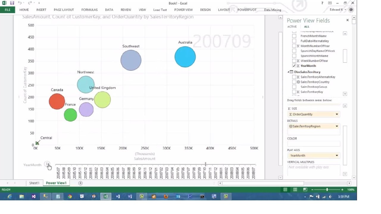
Excel 2013 PowerView Animated Scatterplot/Bubble Chart Business Intelligence Tutorial - YouTube
peltiertech.com › add-horizontal-line-to-excel-chartAdd a Horizontal Line to an Excel Chart - Peltier Tech Sep 11, 2018 · The examples below show how to make combination charts, where an XY-Scatter-type series is added as a horizontal line to another type of chart. Add a Horizontal Line to an XY Scatter Chart. An XY Scatter chart is the easiest case. Here is a simple XY chart.
Scatter Plot in Excel - Easy Excel Tutorial
How to display text labels in the X-axis of scatter chart in Excel? Display text labels in X-axis of scatter chart. Actually, there is no way that can display text labels in the X-axis of scatter chart in Excel, but we can create a line chart and make it look like a scatter chart. 1. Select the data you use, and click Insert > Insert Line & Area Chart > Line with Markers to select a line chart. See screenshot:

Excel: labels on a scatter chart, read from array - Stack Overflow
Change hover label data on Scatter plot chart - MrExcel Message Board Hi, I have 8 scattered plot charts, all containing more than 300 dots.. This means that I cant use ordinary labels, because it destroys all visibility of the chart. So I need to hover the dots to see the label data. This works good but I cant manage to get the names of the items on the hovering label.

Tutorial: Excel Scatter Charts and More | AIChE
What is a 3D Scatter Plot Chart in Excel? - projectcubicle Select the data set that you want to plot on the chart. 2. Go to Insert tab > Charts group > select Scatter chart from the drop-down menu or click on the Insert button from Charts group, then select Scatter chart from the Insert dialog box. 3.
Excel scatter chart using text name - Access-Excel.Tips
How to add labels in bubble chart in Excel? - ExtendOffice To add labels of name to bubbles, you need to show the labels first. 1. Right click at any bubble and select Add Data Labels from context menu. 2. Then click at one label, then click at it again to select it only. See screenshot: 3. Then type = into the Formula bar, and then select the cell of the relative name you need, and press the Enter key.
How to Make a Scatter Chart - ExcelNotes
How to Change Excel Chart Data Labels to Custom Values? 05.05.2010 · When you “add data labels” to a chart series, excel can show either “category” , “series” or “data point values” as data labels. But what if you want to have a data label that is altogether different, like this: You can change data labels and point them to different cells using this little trick. First add data labels to the chart (Layout Ribbon > Data Labels) Define the …

Multiple Series in One Excel Chart - Peltier Tech Blog
Excel Chart Vertical Axis Text Labels • My Online Training Hub So all we need to do is get that bar chart into our line chart, align the labels to the line chart and then hide the bars. We’ll do this with a dummy series: Copy cells G4:H10 (note row 5 is intentionally blank) > CTRL+C to copy the cells > select the chart > CTRL+V to paste the dummy data into the chart.
Excel::Writer::XLSX::Chart::Scatter - A class for writing Excel Scatter charts. - metacpan.org
How to use a macro to add labels to data points in an xy scatter chart ... In Microsoft Excel, there is no built-in command that automatically attaches text labels to data points in an xy (scatter) or Bubble chart. However, you can create a Microsoft Visual Basic for Applications macro that does this. This article contains a sample macro that performs this task on an XY Scatter chart. However, the same code can be ...

Line Graph, Bar Graph, Scatter, Etc. | University of Denver
Excel not letting me change Y axis bounds in scatter chart Excel not letting me change Y axis bounds in scatter chart. Hello, I am having an issue in that excel is not letting me start the Y axis of a scatter plot at a different value to zero. I cannot seem to find an option to turn off the automatic formatting. Any help would be greatly appreciated.
python - Need to use matplotlib scatter markers outside the chart, in labels for a bar graph ...
Excel Scatter Chart - change x-axis labels When I create a Scatter Chart there are numbers along the x-axis. I am using the below data: 2010 2011 North 30 50 South 50 100 East 20 20 West 100 30 Is it possible to change the numbers on the x-axis to display each heading, ie North, South East and West. · One way: Convert the years to text... Yr 2010 Yr 2011 Use a Line chart. Format each series to ...

Scatter Chart in Excel
› easiest-waterfall-chart-in-excelWaterfall Chart in Excel - Easiest method to build. - XelPlus At this point it might look like you’ve ruined your Waterfall. Excel has added another line chart and is using that for the Up/Down bars. Don’t panic. Just right mouse click on any series and go to the Change Series Chart Type… From the Change Series Chart Type… options, find the Data Label Position Series and change it to a Scatter Plot.
How to Make a Scatter Chart - ExcelNotes
VBA Scatter Plot Hover Label | MrExcel Message Board Set ser = ActiveChart.SeriesCollection (1) chart_data = ser.Values chart_label = ser.XValues Set txtbox = ActiveSheet.Shapes ("hover") 'I suspect in the error statement is needed for this. If ElementID = xlSeries Then txtbox.Delete Sheet1.Range ("Ch_Series").Value = Arg1 Txt = Sheet1.Range ("CH_Text").Value
Post a Comment for "40 excel scatter chart with labels"