43 rotate data labels excel chart
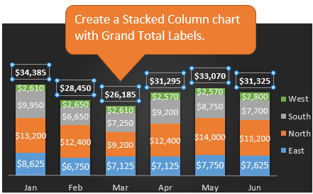
How to: Display and Format Data Labels - DevExpress When data changes, information in the data labels is updated automatically. If required, you can also display custom information in a label. Select the action you wish to perform. Add Data Labels to the Chart. Specify the Position of Data Labels. Apply Number Format to Data Labels. Create a Custom Label Entry. Sunburst Chart in Excel - Example and Explanations The sunburst chart is part of the hierarchical chart family. It allows you to see at a glance the number of hierarchical levels that exist and the proportion that each segment represents... Create a sunburst chart. Creating a sunburst chart is something very simple to do. The only thing The input data just needs to be presented as expected.
How to ☝️Make a Pie Chart in Excel (Free Template) In order to rotate a pie chart without messing up the chart title and legend, do the following: 1. Right-click on your pie chart and pick " Format Data Series " from the menu that appears. 2. Go to the " Series Option " tab. 3.

Rotate data labels excel chart
› how-to-show-percentage-inHow to Show Percentage in Pie Chart in Excel? - GeeksforGeeks Jun 29, 2021 · It can be observed that the pie chart contains the value in the labels but our aim is to show the data labels in terms of percentage. Show percentage in a pie chart: The steps are as follows : Select the pie chart. Right-click on it. A pop-down menu will appear. Click on the Format Data Labels option. The Format Data Labels dialog box will appear. 3D Surface Chart in Excel - Insert, Format, Working - Excel Unlocked We can insert the chart for this data. Follow the below-mentioned steps:-. Select the range of cells A1:F7. Go to the Insert tab on the ribbon and Click on Recommended Charts button. Navigate to All Charts tab and select the Surface Chart from the list down there. Format Chart Axis in Excel - Axis Options Analyzing Format Axis Pane. Right-click on the Vertical Axis of this chart and select the "Format Axis" option from the shortcut menu. This will open up the format axis pane at the right of your excel interface. Thereafter, Axis options and Text options are the two sub panes of the format axis pane.
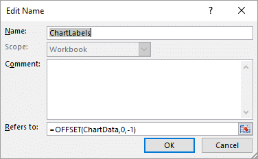
Rotate data labels excel chart. How to: Display and Format Data Labels - DevExpress Add Data Labels to the Chart; Specify the Position of Data Labels; Apply Number Format to Data Labels; Create a Custom Label Entry; Add Data Labels to the Chart. Basic settings that specify the contents, position and appearance of data labels in the chart are defined by the DataLabelOptions object, accessed by the ChartView.DataLabels property ... support.microsoft.com › en-us › officeRotate a pie chart - support.microsoft.com If you want to rotate another type of chart, such as a bar or column chart, you simply change the chart type to the style that you want. For example, to rotate a column chart, you would change it to a bar chart. Select the chart, click the Chart Tools Design tab, and then click Change Chart Type. See Also. Add a pie chart. Available chart types ... How to modify the data for a chart in excel - Basic Excel Tutorial The following steps are involved in the process of changing the chart's labels. 1. Open the excel application. Then, locate the chart you wish to edit on your storage. 2. Click on the chart displayed. And a chart toolbar appears on the top part of the screen. 3. Click on the layout button, located under chart tools. 4. › charts › axis-labelsHow to add Axis Labels (X & Y) in Excel & Google Sheets Edit Chart Axis Labels. Click the Axis Title; Highlight the old axis labels; Type in your new axis name; Make sure the Axis Labels are clear, concise, and easy to understand. Dynamic Axis Titles. To make your Axis titles dynamic, enter a formula for your chart title. Click on the Axis Title you want to change
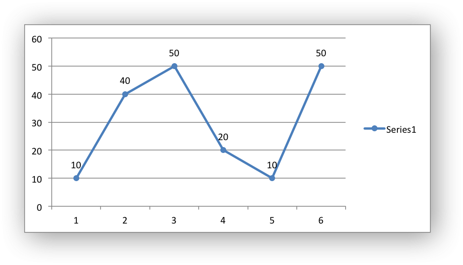
How to Create and Customize a Treemap Chart in Microsoft Excel Either right-click the chart and pick "Format Chart Area" or double-click the chart to open the sidebar. On Windows, you'll see two handy buttons on the right of your chart when you select it. With these, you can add, remove, and reposition Chart Elements. And you can pick a style or color scheme with the Chart Styles button. How to create a step chart in Excel - Excel Off The Grid The Source data inside an Excel chart can be non-contiguous; therefore, we can create a step chart without changing any data at all - Woop, Woop! Create a line chart as usual, using the original data. Right-click on the chart, click Select Data… from the menu. Select the data series and click Edit. Change the series values to be: › 07 › 09Rotate charts in Excel - spin bar, column, pie and line charts Jul 09, 2014 · In my picture below, data labels overlap the title, which makes it look unpresentable. I am going to copy it to my PowerPoint Presentation about peoples' eating habits and want the chart to look well-ordered. To fix the issue and emphasize the most important fact, you need to know how to rotate pie chart in Excel clockwise. Excel Waterfall Chart: How to Create One That Doesn't Suck Ideally, you would create a waterfall chart the same way as any other Excel chart: (1) click inside the data table, (2) click in the ribbon on the chart you want to insert. ... in Excel 2016 Microsoft decided to listen to user feedback and introduced 6 highly requested charts in Excel 2016, including a built-in Excel waterfall chart.
Rotating X-Axis labels so that the end of the label ends on ticks | WPF ... Currently I am using "RotateTransform" in combination with "LayoutTransform" with a negative angle. The labels already rotate, but they rotate around the center of width and size of the label. What I want to achieve is that the rotated label ends on the Tick line of the X-Axis like in Screenshot from an Excel Diagram which is attached ... Pivot chart data labels rotate - Excel Help Forum For a new thread (1st post), scroll to Manage Attachments, otherwise scroll down to GO ADVANCED, click, and then scroll down to MANAGE ATTACHMENTS and click again. Now follow the instructions at the top of that screen. New Notice for experts and gurus: How to Print Labels from Excel - Lifewire Select Mailings > Write & Insert Fields > Update Labels . Once you have the Excel spreadsheet and the Word document set up, you can merge the information and print your labels. Click Finish & Merge in the Finish group on the Mailings tab. Click Edit Individual Documents to preview how your printed labels will appear. Select All > OK . How to make 3 axis graph | Microsoft Excel Tips | Excel Tutorial | Free ... Select the data including labels, in Insert ribbon tab go to column and select 3-D chart. And that's it! You've just inserted 3 axis chart. Right click on bars and select 3-D Rotation to adjust the grade visibility. Note: For learning purpose use the table shown above (numbers in an increasing pattern).
How To Use Dynamic Data Labels To Create Interactive Excel Charts
Excel Dynamic Chart Linked with a Drop-down List - GeeksforGeeks Follow the below steps to implement a dynamic chart linked with a drop-down menu in Excel: Step 1: Insert the data set into an Excel sheet in the cells as shown above. Step 2: Now select any cell where you want to create the drop-down list for the courses. Step 3: Now click on the Data tab from the top of the Excel window and then click on Data ...
Create a Rolling Chart for Last 6 Months | Microsoft Excel Tips and Tricks - Computergaga
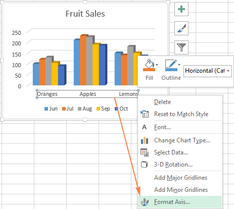
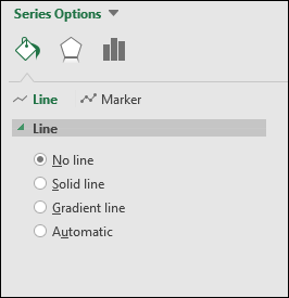
How to make shading on Excel chart and move x axis labels to the bottom ... In the Change Chart Type dialog, change the chart type for the new series to Stacked Area. Change the color from whatever Excel decides to yellow. Finally, remove the new series form the legend. See the attached version. Wi-Fi Signal Strength.xlsx 15 KB 0 Likes Reply Snoopdon replied to Hans Vogelaar Oct 24 2021 05:18 PM
Working with Charts — XlsxWriter Documentation
› 509290 › how-to-use-cell-valuesHow to Use Cell Values for Excel Chart Labels Mar 12, 2020 · Select the chart, choose the “Chart Elements” option, click the “Data Labels” arrow, and then “More Options.” Uncheck the “Value” box and check the “Value From Cells” box. Select cells C2:C6 to use for the data label range and then click the “OK” button.

Dot Plots in Microsoft Excel - Peltier Tech Blog
Position labels in a paginated report chart - Microsoft Report Builder ... To change the position of point labels in a Bar chart Create a bar chart. On the design surface, right-click the chart and select Show Data Labels. Open the Properties pane. On the View tab, click Properties On the design surface, click the chart. The properties for the chart are displayed in the Properties pane.
Excel Bar Chart X Axis Values - using columns and bars to compare items in excel charts ...
DataLabel.Position property (Excel) | Microsoft Docs DataLabel object Properties DataLabel.Position property (Excel) Article 09/13/2021 2 minutes to read 6 contributors In this article Syntax Returns or sets an XlDataLabelPosition value that represents the position of the data label. Syntax expression. Position expression A variable that represents a DataLabel object. Support and feedback

Rotate Pie Chart in Excel | How to Rotate Pie Chart in Excel?
excel - Formatting Data Labels on a Chart - Stack Overflow sub charttest () activesheet.chartobjects ("chart 6").activate z = 1 with activechart if .charttype = xlline then i = .seriescollection (1).points.count activechart.fullseriescollection (1).datalabels.select for pts = 1 to i activechart.fullseriescollection (1).points (pts).hasdatalabel = true ' make sure all points are visible data …

E-xcel Tuts: Add Data Labels to Excel Charts
› charts › timeline-templateHow to Create a Timeline Chart in Excel - Automate Excel Right-click on any of the columns representing Series “Hours Spent” and select “Add Data Labels.” Once there, right-click on any of the data labels and open the Format Data Labels task pane. Then, insert the labels into your chart: Navigate to the Label Options tab. Check the “Value From Cells” box.
EXCEL Charts: Column, Bar, Pie and Line
Rotate Axis Labels of Base R Plot - GeeksforGeeks Rotate axis labels perpendicular to the axis. In this example, we will be rotating the axis labels of the base R plot of 10 data points same as used in the previous example to the perpendicular position by the use of the plot function with the las argument with its value as 2 in the R programming language. R. x = c(2, 7, 9, 1, 4, 3, 5, 6, 8, 10)
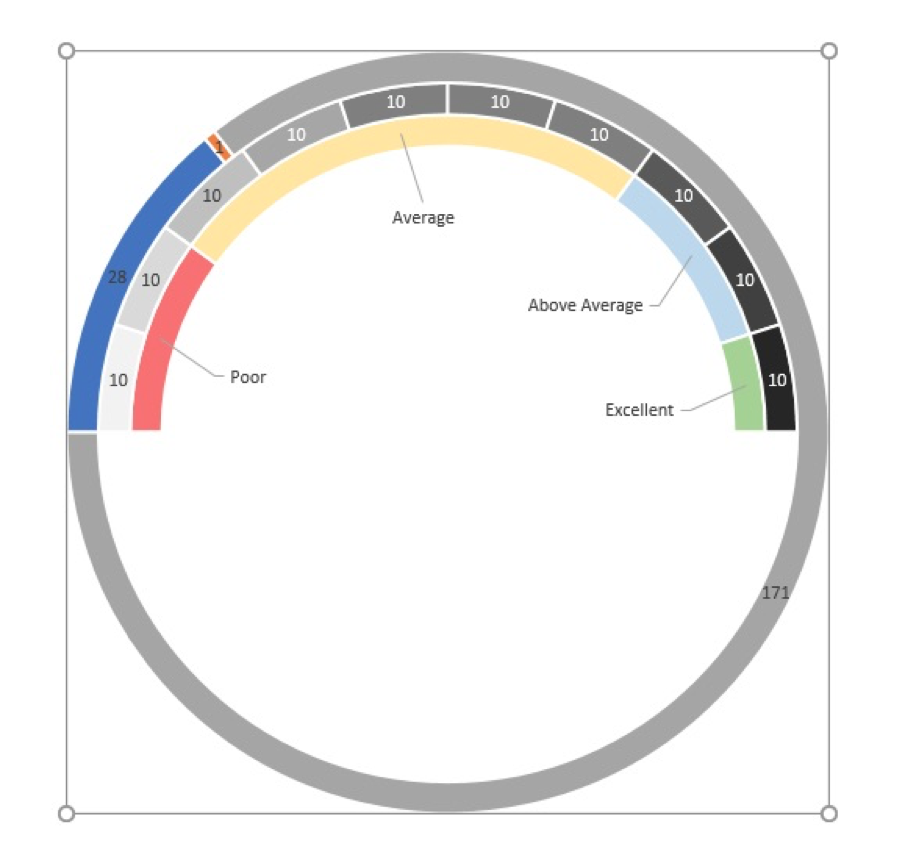
How To Build Gorgeous Speedometer Charts and Why You Shouldn't Use Them - I Will Teach You Excel
How to plot a pie chart in Excel | Basic Excel Tutorial 1. On your computer, open the worksheet you want to create a pie chart. 2. In your spreadsheet, select the range of data you want to use for your pie chart. 3. On the main menu ribbon, click on the Insert tab. 4. Here you will see different types of charts, click on the Pie chart icon drop-down arrow. From the list, pick the chart you want. 5.

Rotate charts in Excel 2010-2013 – spin bar, column, pie and line charts
Using Text Rotation to Create Custom Table Headers in Google Sheets Rotate up - rotate the text 90° up; Rotate down - rotate the text 90° down ... Here's an example showing a diagonal line to separate the row and column heading labels in a single cell: To achieve this, use the CHAR ... like pivot tables or charts. Generally, labels in column A need their own column heading. Alternative Way To Subdivide ...

World Polls Chart -very nicely done chart to combine multiple data sets. Free excel chart ...
Matplotlib Bar Chart Labels - Python Guides Read: Matplotlib scatter marker Matplotlib bar chart labels vertical. By using the plt.bar() method we can plot the bar chart and by using the xticks(), yticks() method we can easily align the labels on the x-axis and y-axis respectively.. Here we set the rotation key to "vertical" so, we can align the bar chart labels in vertical directions.. Let's see an example of vertical aligned labels:
Create Dynamic Chart Data Labels with Slicers - Excel Campus
How to Create Exploding Pie Charts in Excel - Lifewire Click the Insert tab of the ribbon . In the Charts box of the ribbon, click the Insert Pie Chart icon to open the drop-down menu of available chart types. Hover your mouse pointer over a chart type to read a description of the chart. Click either Pie of Pie or Bar of Pie chart in the 2-D Pie section of the drop-down menu to add that chart to ...
How To Use Dynamic Data Labels To Create Interactive Excel Charts
How to create pill charts in Excel - SpreadsheetWeb Click on Starting Space parts on the column chart. Make sure each of them is selected. Right-click on them and select No Fill as a Fill color. Apply same approach for the Ending Spaces as well. These invisible spaces gives enough gaps for hovering affect. 4. Rounding Edges This is where magic happens.

3 Bar Graph In Excel - Free Table Bar Chart
Two-Level Axis Labels (Microsoft Excel) Excel automatically recognizes that you have two rows being used for the X-axis labels, and formats the chart correctly. Since the X-axis labels appear beneath the chart data, the order of the label rows is reversed—exactly as mentioned at the first of this tip. (See Figure 1.) Figure 1. Two-level axis labels are created automatically by Excel.

Finish: Chart | Basics | Jan's Working with Numbers
How to Apply a Filter to a Chart in Microsoft Excel Select the data for your chart, not the chart itself. Go to the Home tab, click the Sort & Filter drop-down arrow in the ribbon, and choose "Filter." Click the arrow at the top of the column for the chart data you want to filter. Use the Filter section of the pop-up box to filter by color, condition, or value.

32 How To Label Graphs In Excel - Labels Database 2020
support.microsoft.com › en-us › officePresent your data in a doughnut chart - support.microsoft.com On the Design tab, in the Chart Layouts group, select the layout that you want to use.. For our doughnut chart, we used Layout 6.. Layout 6 displays a legend. If your chart has too many legend entries or if the legend entries are not easy to distinguish, you may want to add data labels to the data points of the doughnut chart instead of displaying a legend (Layout tab, Labels group, Data ...
Post a Comment for "43 rotate data labels excel chart"